Interpretation of the results of GIMIC calculations
For the thorough interpretation of the induced current densities in a molecule it is recommended to do both visual and quantitative investigation. It is recommended to get a feeling of the molecule by running 3D calculations first. After that, one can choose suitable locations for the integration planes that will quantify the observed vortices.
It is important to keep that when placing an integration plane, we can only determine whether the current flow to the left or to the right at each grid point. This is caused by the fact that tropicity is a non-local property - i.e. one needs to follow streamlines obtained with path integration in order to determine whether the current flow is clockwise (diatropic) or counterclockwise (paratropic) with respect to the magnetic field vector. When integrating through a whole benzene molecule, there are two symmetric pairs of positive and negative contributions exactly because the current flow on one side of the vortex origin is going to the left with respect to the integration plane and in then as it returns, it looks as if it is flowing to the right. One needs topology analysis, which is not part of our code. We tackle the issue by applying some intuition. We know that inside every molecular ring there should be paratropic current, which we call negative simply out of convention. Then we know that around every molecule (aromatic, non-aromatic, or antiaromatic) there is a diatropic current, which we call positive.
We have a Youtube channel showing some of the basics: https://www.youtube.com/channel/UC_5dN4qhYTOtr-itnsjoE0w/videos.
3D integration
A current density calculation can be performed using the cdens set of
keywords in the input file. It is possible to use the interactive script called
3D-run.sh to define a box around the molecule and specify the distance
between the grid points. We recommend to use Paraview to visualise the results
(https://www.paraview.org/). Our recommended setup for Paraview can be seen in
this video (https://www.youtube.com/watch?v=NngG1g3Bb7Q&t=5s).
The jvec.vti files is what concerns us the most. Also, it is necessary to
convert the molecular coordinates to CML format and bohr units. This is easily
done using the bash function molecule given in the description of the
section on the interactive scripts.
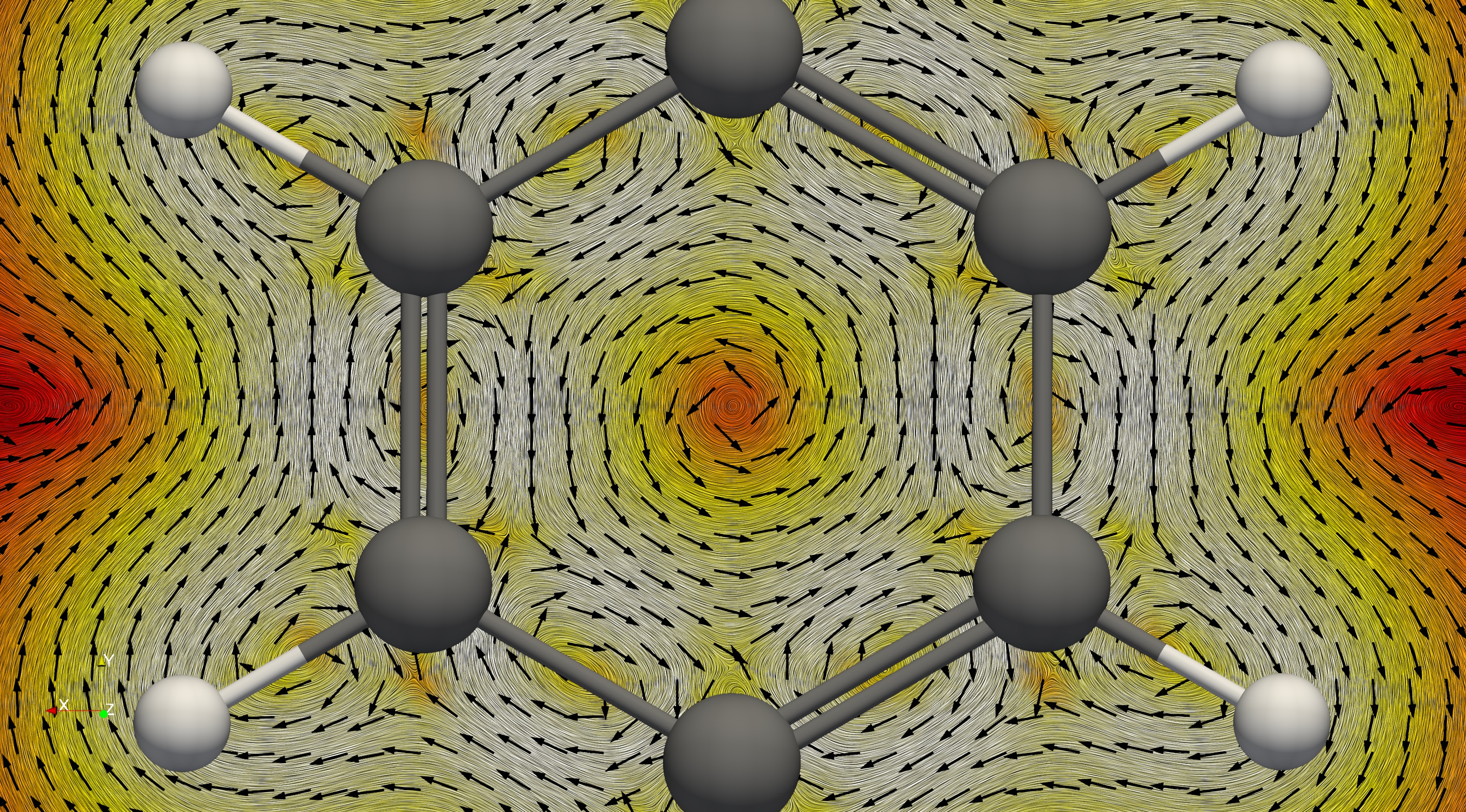
It is possible to do streamline plots using the StreamTracer tool. Slices on a plane can be done using the Surface LIC (line integral convolution) plug-in to show the direction of the current flow.
Streamline (spaghetti) plots

In this video (https://www.youtube.com/watch?v=Pjy_0jucmGQ&t=28s) we present in short how to create the streamline “spaghetti” plots using Paraview. A pre-requisite is to have performed a current density calculations and that the jvec.vti and mol-bohr.cml files exist. The latter is not directly written by GIMIC but in the documentation we have suggested a bash function which creates it.
After the two files are loaded on the blank board we see the molecule and a rectangular object which shows the boundaries of the defined integration grid for the calculation. Then we apply the Stream Tracer tool. What is does is to define some points in space and calculates their trajectory as if they were particles moving in the vector field. It simply does path integration along the direction defined by the vector field at each point. By default it uses a line (High Resolution Line Source) as a seed type. It has to be changed to Point Source from the drop-down menu. The next step is to change the radius of the sphere. Usually a small sphere works better to distinguish different current loops. The length of the field line can be defined to match the size of the molecule. An important parameter is the Integration Direction. Forward or backward directions can be used to visually determine the tropicity of the current flow. One needs to check the magnetic field direction defined in the calculation and then look at the molecule along that axis. For example when the field points to the negative Z direction, then one needs to rotate the molecule, so that the view is towards the negative Z axis. Setting forward integration direction produces the correct tropicity direction according to the convention. It is accepted that diatropic current flow clockwise, while paratropic currents - counterclockwise. In any molecule on the outside, far from the nuclei, there is diatropic flow with strength determined by the magnetic response. Also, in the vicinity of the atomic nuclei there also are diatropic currents flowing clockwise. Inside molecular rings there is a paratropic counterclockwise current pathway, irrespective of whether the ring is aromatic or antiaromatic.
It appears that our job is already finished here, however we have not considered yet the current strength. Many of the curves turn out to be very weak and negligible. The lines can be made thicker by applying the Tube filter and a suitable colour scheme can be set with a suitable range of values. We typically use the Blackbody radiation scheme with range [1e-6; 0.1], however based on the particular investigated molecule the range may need to be adjusted. With that done one can freely explore the streamlines in the molecule. It is sometimes useful to make a very small sphere but with many points. When the result looks good the view can be saved as PNG, for example. It is recommended to export high-resolution images with high quality compression in case of JPG format.
Integration planes
Current profile integration
In this video we present how to interactively calculate a current profile across a bond in GIMIC. We start off in a directory where the nuclear shielding calculation for the benzene molecule has been executed with Turbomole.
The molecular coordinates can be previewed by converting the TURBOMOLE coord file to XYZ format using the t2x program. In this example we show the coordinates in the basic XMAKEMOL program. It is lightweight and works over SSH smoothly. XMAKEMOL loads a molecule showing hydrogen bonds as dashed lines. They can be turned off by pressing the H key on the keyboard. The atomic indices can be shown by pressing the N key. The latter is needed for the definition of the integration plane. Zooming in closer can be done by pressing CTRL + P. The first slider changes the zoom level. The “Toggle depth” option switches between perspective and orthographic projection of the atoms. XMAKEMOL can be downloaded from http://www.nongnu.org/xmakemol. Please note that we are not affiliated or contributing to the development of XMAKEMOL in any way. Of course, one can use any other molecular visualisation program, such as Molden or VMD.
When we have inspected the molecular geometry and selected the bond through which to place an integration plane, it is time to prepare the gimic input files. The files CAODENS and XCAODENS contain the unperturbed and the magnetically perturbed density matrices. If they are missing, then the nuclear shielding calculation did not complete. They are converted to the file XDENS using the Python script turbo2gimic.py. It is handy to define it as a bash alias. Please pipe the output to the file called MOL.
With that done, the current profile script can be called. In this example we show the version for a cluster, however, it can be used in the same manner on a local machine. It is good to remember that GIMIC works in atomic units. We have decided to integrate the current in the benzene molecule. This can be done by placing an integration plane across any of the C = C bonds. The bond is defined using the indices of the atoms according to the coord file. XMAKEMOL makes the choice easy by displaying the indices. NOTE to VMD users! The first atom in the XYZ file has the index one. VMD lists the indices starting from 0, so the given index needs to be increase by one. In this example we chose to integrate across the bond between atoms 4 and 5. According to our convention the atoms are entered in clockwise order, i.e. 4 – 5 instead of 5 – 4 in this case. The scripts asks for a possible suffix for the directory name. This can be generally omitted, however sometimes it might be necessary to run calculations across the same bond but along different integration planes. In practice this means that if the suffix “modified” is entered, then the created calculation directory is current_profile_4.5_modified.
Next, we need to define at which point the bond and the integration plane cross. Unless there is a particular reason, we set the plane to cross the midpoint of the bond. Possible reasons to shift it would be, for example, additional current vortices, which might interfere with the estimation of the currents.
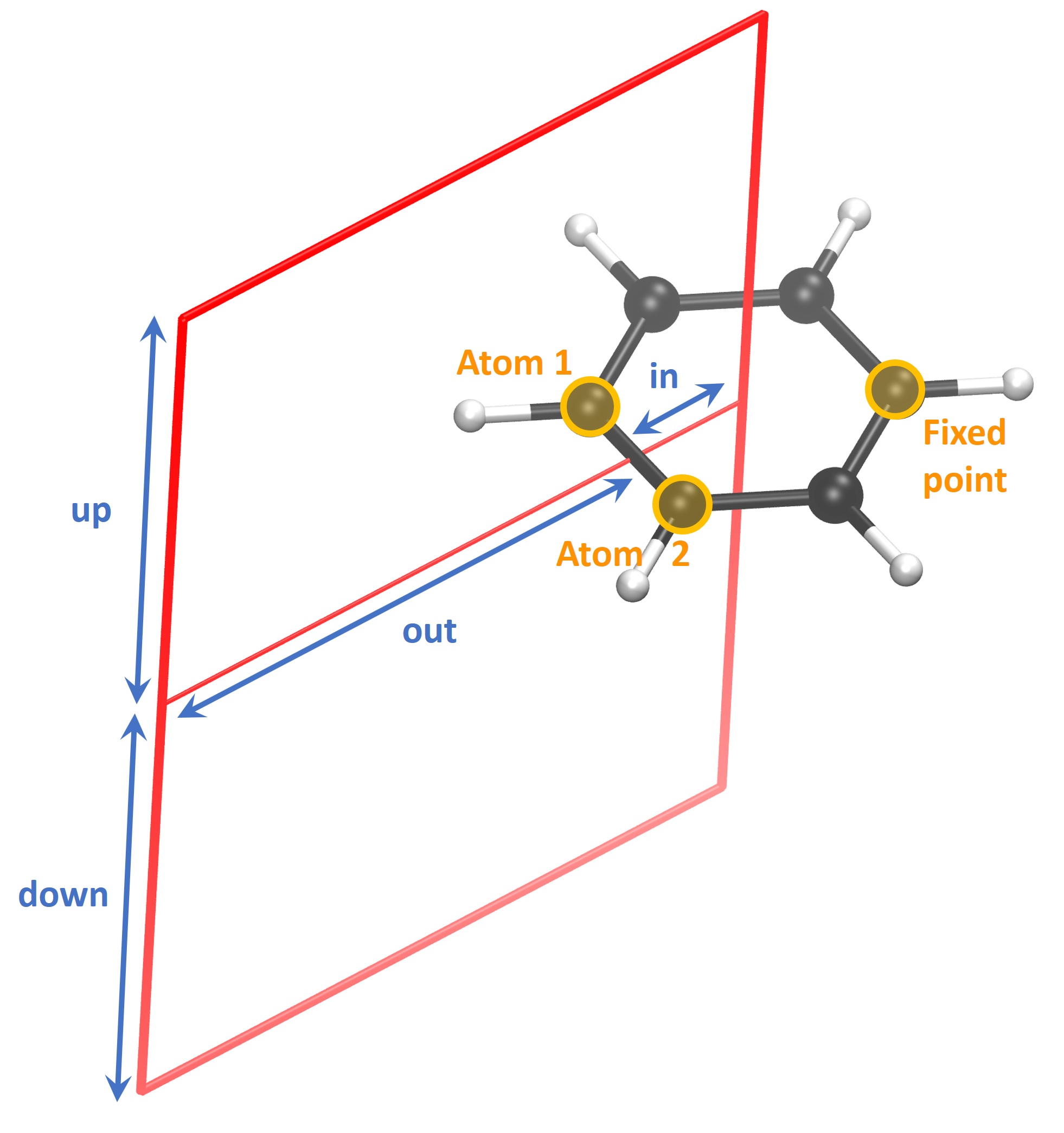
Then the integration plane has to be positioned in space. Integration always occurs from right to left, so keep that in mind when defining the in and out distances. The in value can be defined either by specifying atomic indices or by choosing a certain value away from the bond. In the presented case we chose to integrate from the centre of the ring to infinity. Clearly, in this case it is easier to define the starting point through the indices of three atoms. This is done by entering the indices in arbitrary order but on the same line. The geometrical centroid of the hexagon is printed. For symmetric molecules, such as benzene, this is a good starting point. Otherwise, it is recommended to increase the distance a bit since the current vortex is not symmetric, either. In this example we increase the value by about 0.15 bohr. We want the end point to be infinitely far away from the molecule, where the current vanished. Practice has shown that usually at 8 bohr away from the bond, the current reaches 0. Similarly, we integrate infinitely far above and below the molecule by setting the up and down values to 8 bohr.
The next steps is to specify the thickness of the slices. We recommend to use 0.02 bohr to produce a nice high-resolution plot. Each slice is executed as a separate calculation. Grid point spacing refers to the grid for each slice. The pre-defined values have proven to yield good results.
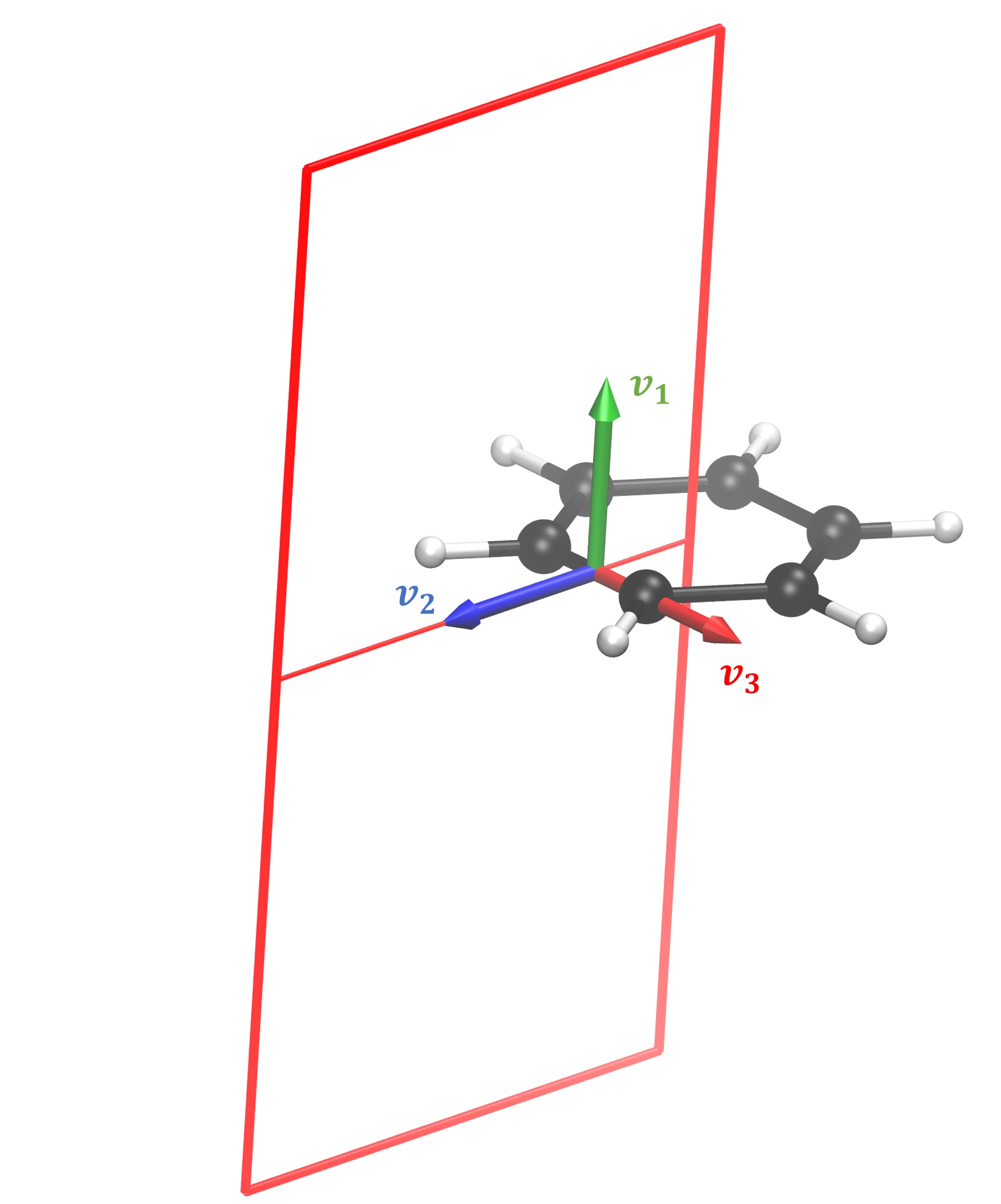
The magnetic field direction can be specified in several different ways. The strongest currents are induced when the field is perpendicular to the molecular ring. Traditionally, molecules are placed to lie in the xy plane, thus the magnetic field vector B = (0; 0; -1). In some cases it is necessary to rotate the field with respect to the integration plane. For example, bond currents can be calculated by setting B = (-1; 0; 0) in the chosen example, so that the field is perpendicular to the bond but lies in the plane of the benzene molecule. However, this definition of B || X, Y or Z can be overridden. If the molecule was not placed in the xy plane, and particularly in non-planar molecules, it is best to define the atoms with respect to which the field will be perpendicular. The tools maximize_projection and plane in the GIMIC repository need to be available for the automatic calculation of the field vector.
Afterwards, it is necessary to define the “fixed point”. It is the third point which specifies the integration plane. The script attempts to calculate it, however, it sometimes fails. In those cases, one needs to manually try and choose an atom which is located clockwise with respect to the bond atoms (4 and 5 in this example). Having done that, one can further rotate the integration plane if needed. It can be done by entering an angle in degrees. By default, the origin of rotation is the bond midpoint, however, the origin can be modified if needed.
The script prints a summary of the defined integration plane and performs a dry run for the first slice of the integration plane.
(to be continued, and the video has to be finished)